How to Read Ordinal Logistic Fit Analysis in Jmp

Version info: Code for this page was tested in IBM SPSS 20.

Please note: The purpose of this page is to prove how to use various information analysis commands. It does not encompass all aspects of the research process which researchers are expected to do. In particular, it does not cover data cleaning and checking, verification of assumptions, model diagnostics and potential follow-up analyses.

Examples of ordered logistic regression

Example 1: A marketing research firm wants to investigate what factors influence the size of soda (small, medium, large or actress large) that people order at a fast-food chain. These factors may include what type of sandwich is ordered (burger or chicken), whether or not fries are likewise ordered, and age of the consumer. While the outcome variable, size of soda, is obviously ordered, the divergence between the diverse sizes is non consequent. The divergence betwixt small-scale and medium is x ounces, between medium and big eight, and between large and extra large 12.

Case two: A researcher is interested in what factors influence medaling in Olympic swimming.  Relevant predictors include at training hours, diet, historic period, and popularity of swimming in the athlete's home country. The researcher believes that the distance between gilt and silver is larger than the distance between silver and bronze.

Case 3: A report looks at factors that influence the conclusion of whether to apply to graduate school.  College juniors are asked if they are unlikely, somewhat likely, or very probable to use to graduate school. Hence, our result variable has three categories. Information on parental educational status, whether the undergraduate institution is public or private, and current GPA is also collected. The researchers accept reason to believe that the "distances" between these three points are not equal.  For example, the "altitude" between "unlikely" and "somewhat likely" may be shorter than the distance between "somewhat probable" and "very likely".

Clarification of the data

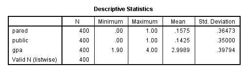
For our data assay below, we are going to expand on Example 3 about applying to graduate school. We accept simulated some data for this example and it can be obtained from here: ologit.sav This hypothetical data set has a three-level variable called apply (coded 0, i, 2), that we will use every bit our outcome variable. We also have three variables that we will utilise as predictors: pared, which is a 0/one variable indicating whether at to the lowest degree one parent has a graduate degree; public, which is a 0/i variable where 1 indicates that the undergraduate institution is public and 0 individual, and gpa, which is the educatee's course point average.

Permit's commencement with the descriptive statistics of these variables.

                                  get file "D:\data\ologit.sav". freq var = use pared public.                                descriptives var = gpa.                              

Analysis methods you might consider

Beneath is a list of some analysis methods you may have encountered. Some of the methods listed are quite reasonable while others accept either fallen out of favor or have limitations.

• Ordered logistic regression: the focus of this page.
• OLS regression: This analysis is problematic because the assumptions of OLS are violated when information technology is used with a non-interval outcome variable.
• ANOVA: If you use only one continuous predictor, you could "flip" the model around so that, say, gpa was the outcome variable and apply was the predictor variable. Then you could run a one-manner ANOVA. This isn't a bad thing to do if you simply have 1 predictor variable (from the logistic model), and it is continuous.
• Multinomial logistic regression:  This is similar to doing ordered logistic regression, except that it is causeless that there is no order to the categories of the outcome variable (i.e., the categories are nominal). The downside of this approach is that the information contained in the ordering is lost.
• Ordered probit regression: This is very, very similar to running an ordered logistic regression. The main divergence is in the interpretation of the coefficients.

Ordered logistic regression

Before we run our ordinal logistic model, we will see if whatever cells are empty or extremely small.  If whatsoever are, we may have difficulty running our model. At that place are two ways in SPSS that nosotros tin can do this.  The starting time way is to make simple crosstabs.  The second way is to use the cellinfo pick on the /print subcommand.  Yous should use the cellinfo option just with categorical predictor variables; the table volition exist long and difficult to translate if you include continuous predictors.

              crosstabs /tables = employ by pared /tables = apply by public.                            plum use with pared public  /link = logit /impress = cellinfo.                          

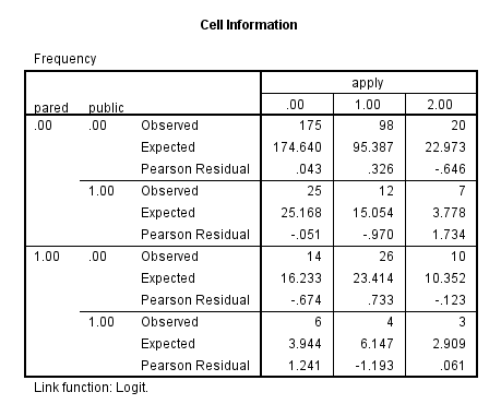
None of the cells is too minor or empty (has no cases), so we will run our model. In the syntax below, we accept included the link = logit subcommand, even though information technology is the default, just to remind ourselves that we are using the logit link part. Also note that if y'all do not include the impress subcommand, merely the Case Processing Summary table is provided in the output.

              plum apply with pared public gpa /link = logit /print = parameter summary.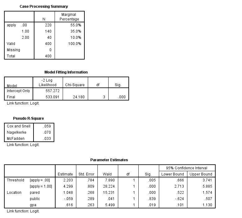                                        

In the Case Processing Summary table, nosotros see the number and percentage of cases in each level of our response variable. These numbers await fine, but nosotros would exist concerned if i level had very few cases in information technology. We as well see that all 400 observations in our data set were used in the analysis. Fewer observations would have been used if whatever of our variables had missing values. By default, SPSS does a listwise deletion of cases with missing values.  Next we see the Model Plumbing equipment Information table, which gives the -2 log likelihood for the intercept-only and terminal models. The -2 log likelihood can be used in comparisons of nested models, just we won't show an example of that here.

In the Parameter Estimates table we see the coefficients, their standard errors, the Wald test and associated p-values (Sig.), and the 95% confidence interval of the coefficients. Both pared and gpa are statistically significant; public is not.& And so for pared, we would say that for a 1 unit increment in pared (i.e., going from 0 to 1), nosotros expect a 1.05 increment in the ordered log odds of being in a higher level of apply, given all of the other variables in the model are held abiding. For gpa, we would say that for a one unit increment in gpa, we would expect a 0.62 increase in the log odds of existence in a higher level of use, given that all of the other variables in the model are held constant. The thresholds are shown at the top of the parameter estimates output, and they betoken where the latent variable is cutting to brand the three groups that we notice in our data. Note that this latent variable is continuous. In general, these are not used in the estimation of the results. Some statistical packages phone call the thresholds "cutpoints" (thresholds and cutpoints are the same thing); other packages, such as SAS study intercepts, which are the negative of the thresholds. In this example, the intercepts would exist -two.203 and -four.299. For farther information, delight see the Stata FAQ: How can I catechumen Stata's parameterization of ordered probit and logistic models to one in which a abiding is estimated?

As of version fifteen of SPSS, you cannot direct obtain the proportional odds ratios from SPSS. You tin can either use the SPSS Output Direction Organization (OMS) to capture the parameter estimates and exponentiate them, or you can calculate them by hand. Please see Ordinal Regression by Marija J. Norusis for examples of how to do this. The commands for using OMS and calculating the proportional odds ratios is shown below. For more information on how to employ OMS, please see our SPSS FAQ: How can I output my results to a data file in SPSS? Please annotation that the single quotes in the square brackets are important, and y'all will get an mistake message if they are omitted or unbalanced.

                oms select tables  /destination format = sav outfile = "D:\ologit_results.sav"  /if commands = ['plum'] subtypes = ['Parameter Estimates'].  plum utilize with pared public gpa /link = logit /print = parameter.  omsend.  get file "D:\ologit_results.sav". rename variables Var2 = Predictor_Variables. * the side by side command deletes the thresholds from the data set. select if Var1 = "Location". exe. * the command below removes unnessary variables from the data set. * transformations cannot be pending for the command below to work, so * the exe. * higher up is necessary. delete variables Command_ Subtype_ Label_ Var1. compute expb = exp(Estimate). compute Lower_95_CI = exp(LowerBound). compute Upper_95_CI = exp(UpperBound). execute.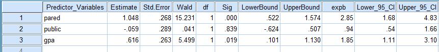                                              

In the column expb nosotros meet the results presented as proportional odds ratios (the coefficient exponentiated). Nosotros take also calculated the lower and upper 95% conviction interval. We would interpret these pretty much as we would odds ratios from a binary logistic regression. For pared, we would say that for a one unit increase in pared, i.east., going from 0 to 1, the odds of high utilise versus the combined center and low categories are 2.85 greater, given that all of the other variables in the model are held constant. Likewise, the odds of the combined heart and loftier categories versus low apply is 2.85 times greater, given that all of the other variables in the model are held constant. For a one unit increase in gpa, the odds of the low and center categories of apply versus the loftier category of apply are i.85 times greater, given that the other variables in the model are held constant. Because of the proportional odds supposition (see beneath for more than explanation), the aforementioned increase, 1.85 times, is plant between low apply and the combined categories of centre and high apply.

One of the assumptions underlying ordered logistic (and ordered probit) regression is that the relationship between each pair of outcome groups is the same. In other words, ordered logistic regression assumes that the coefficients that depict the relationship between, say, the lowest versus all higher categories of the response variable are the same as those that draw the relationship between the next everyman category and all higher categories, etc. This is called the proportional odds assumption or the parallel regression supposition. Considering the relationship between all pairs of groups is the same, there is only one prepare of coefficients (only one model). If this was non the case, we would need different models to describe the relationship betwixt each pair of outcome groups. Nosotros need to test the proportional odds supposition, and we tin can use the tparallel choice on the print subcommand. The null hypothesis of this chi-square exam is that there is no divergence in the coefficients between models, then we hope to get a not-pregnant result.

                plum apply with pared public gpa /link = logit /print = tparallel.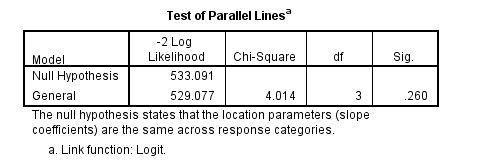                              

The above test indicates that we have not violated the proportional odds assumption. If the proportional odds assumption was violated, we may desire to get with multinomial logistic regression.

We we utilize these formulae to calculate the predicted probabilities for each level of the outcome, utilise. Predicted probabilities are usually easier to understand than the coefficients or the odds ratios.

$$P(Y = ii) = \left(\frac{one}{1 + e^{-(a_{2}+b_{1}x_{i} + b_{2}x_{2} + b_{three}x_{3})}}\right)$$ $$P(Y = ane) = \left(\frac{1}{1 + east^{-(a_{1}+b_{1}x_{1} + b_{2}x_{2} + b_{3}x_{3})}}\right) – P(Y = 2)$$ $$P(Y = 0) = 1 – P(Y = 1) – P(Y = ii)$$

We will calculate the predicted probabilities using SPSS' Matrix linguistic communication. We will use pared as an example with a categorical predictor. Hither we will see how the probabilities of membership to each category of apply change every bit we vary pared and hold the other variable at their means. As you can run into, the predicted probability of being in the lowest category of employ is 0.59 if neither parent has a graduate level education and 0.34 otherwise. For the middle category of apply, the predicted probabilities are 0.33 and 0.47, and for the highest category of apply, 0.078 and 0.196 (annotations were added to the output for clarity). Hence, if neither of a respondent's parents accept a graduate level instruction, the predicted probability of applying to graduate school decreases. Note that the intercepts are the negatives of the thresholds. For a more detailed explanation of how to translate the predicted probabilities and its relation to the odds ratio, please refer to FAQ: How practice I interpret the coefficients in an ordinal logistic regression?

                Matrix. * intercept1 intercept2 pared public gpa. * these coefficients are taken from the output. compute b = {-two.203 ; -4.299 ; 1.048 ; -.059 ; .616}. * overall pattern matrix including means of public and gpa. compute x = {{0, 1, 0; 0, 1, 1}, make(2, i, .1425), make(two, 1, 2.998925)}. compute p3 = 1/(one + exp(-10 * b)). * overall pattern matrix including ways of public and gpa. compute x = {{one, 0, 0; 1, 0, 1}, brand(2, 1, .1425), brand(2, i, 2.998925)}. compute p2 = (1/(1 + exp(-x * b))) - p3. compute p1 = make(NROW(p2), ane, 1) - p2 - p3. compute p = {p1, p2, p3}. print p / FORMAT = F5.iv / title = "Predicted Probabilities for Outcomes 0 i 2 for pared 0 1 at means". End Matrix.  Run MATRIX procedure:    Predicted Probabilities for Outcomes 0 i two for pared 0 1 at ways  		(apply=0) 	(use=1)	(utilise=ii) (pared=0)	.5900 		.3313 		.0787  (pared=one)	.3354 		.4687 		.1959    ------ Terminate MATRIX -----                              

Below, we run into the predicted probabilities for gpa at 2, 3 and four. Yous tin see that the predicted probability increases for both the middle and highest categories of apply every bit gpa increases (annotations were added to the output for clarity). For a more than detailed caption of how to interpret the predicted probabilities and its relation to the odds ratio, please refer to FAQ: How practice I interpret the coefficients in an ordinal logistic regression?

              Matrix. * intercept1 intercept2 pared public gpa. * these coefficients are taken from the output. compute b = {-ii.203 ; -4.299 ; 1.048 ; -.059 ; .616}. * overall pattern matrix including means of pared and public. compute x = {make(iii, one, 0), make(3, 1, 1), brand(3, one, .1575), brand(3, 1, .1425), {2; three; iv}}. compute p3 = 1/(1 + exp(-x * b)). * overall design matrix including means of pared and public. compute 10 = {make(3, 1, ane), make(three, 1, 0), make(3, 1, .1575), make(3, ane, .1425), {2; 3; 4}}. compute p2 = (1/(1 + exp(-x * b))) - p3. compute p1 = make(NROW(p2), ane, i) - p2 - p3. compute p = {p1, p2, p3}. impress p / FORMAT = F5.4 / championship = "Predicted Probabilities for Outcomes 0 one two for gpa 2 3 four at means". End Matrix.  Run MATRIX process:    Predicted Probabilities for Outcomes 0 i 2 for gpa two 3 iv at means  		(apply=0) 	(utilise=1)	(apply=two) (gpa=2) 	.6930 		.2553 		.0516  (gpa=3) 	.5494 		.3590 		.0916  (gpa=iv) 	.3971 		.4456 		.1573   ------ Stop MATRIX -----                          

Things to consider

• Perfect prediction: Perfect prediction ways that 1 value of a predictor variable is associated with only one value of the response variable. If this happens, Stata will usually issue a note at the top of the output and will drop the cases so that the model tin run.
• Sample size: Both ordered logistic and ordered probit, using maximum likelihood estimates, require sufficient sample size.  How big is big is a topic of some debate, but they almost ever crave more cases than OLS regression.
• Empty cells or small cells: You should check for empty or modest cells by doing a crosstab between categorical predictors and the outcome variable. If a cell has very few cases, the model may become unstable or it might non run at all.
• Pseudo-R-squared:  In that location is no exact analog of the R-squared institute in OLS.  At that place are many versions of pseudo-R-squares.  Please run across Long and Freese 2005 for more details and explanations of diverse pseudo-R-squares.
• Diagnostics:  Doing diagnostics for non-linear models is difficult, and ordered logit/probit models are even more difficult than binary models.

References

• Agresti, A. (1996) An Introduction to Categorical Information Analysis. New York: John Wiley & Sons, Inc
• Agresti, A. (2002) Chiselled Data Analysis, Second Edition. Hoboken, New Bailiwick of jersey: John Wiley & Sons, Inc.
• Liao, T. F. (1994) Interpreting Probability Models:  Logit, Probit, and Other Generalized Linear Models. Thousand Oaks, CA: Sage Publications, Inc.
• Powers, D. and Xie, Yu. Statistical Methods for Categorical Information Analysis.  Bingley, UK: Emerald Group Publishing Limited.

gilmorevaccom.blogspot.com

Source: https://stats.oarc.ucla.edu/spss/dae/ordinal-logistic-regression/

Share this post